Tidyverse 1: Data wrangling

Setting up a Project

The first thing you should do when you start a new project is to create a new project in RStudio. This will keep all of your files and data in one place, and easy to find later.

[!NOTE]

What is a project?

A project is a way to organize your work in RStudio. It keeps all of your files and data in one place, and makes it easy to find later. You should create a new project for each new project you start. For this class, feel free to use the same project for all of the lessons.

This will also create a new folder on your computer where all of your stuff lives, and you should know how to find it outside of RStudio. If you’re using the class server, the folder will be on a university computer, and you won’t have access to it outside of RStudio.

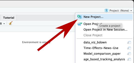
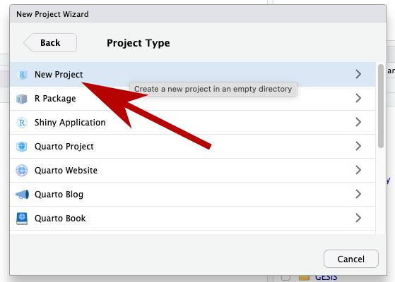
To create a new project, go to “Project” in the upper right hand pane and select > “New Project”.

You should save it in a new directory (another word for folder).

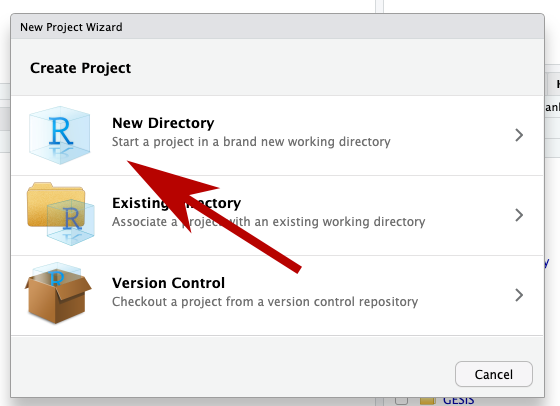
You’ll be presented with a list of options, but for this class I’d go with “New Project”.

Finally, You can call it whatever you like and save it wherever you like, but I suggest something like “data-viz-class”, and maybe put it in your “Documents” folder.

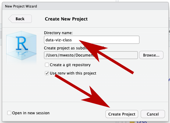
Now hit “Create Project”, and we can start!

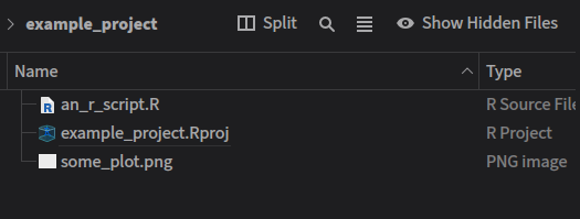
Making a new file

Every time we write a program in R, we should put it in its own file. A good first step for today’s work is to make a new R script via:

File > New File > R Script

Give it a name you’ll remember later like week_1_intro.R

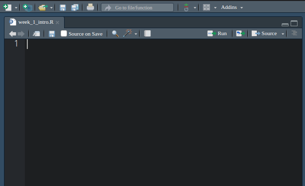
This is … just an empty text file. Very underwhelming. But this is where we’re going to write our code, and make some interesting things happen.

Loading the Tidyverse package

For this class, we’re going to use a package called the Tidyverse. This is a collection of packages that make it easier to work with data. For this, and all of our classes, you’ll want to add this line to the beginning of your script:

[!NOTE]

What is the Tidyverse?

The tidyverse is “… an opinionated collection of R packages designed for data science. All packages share an underlying design philosophy, grammar, and data structures.”

R has always been one of the best tools for doing statistics, but handling the actual data was always kind of a mess, and this largely fixes it. Simply put, it makes R much better at doing data science, and is easily my favorite tool in this space.

Running code

Now, we’ve written our first line of code. But how to run it? You have two options.

• First is to use the “Run” button at the top of the script. This will run the line of code that your cursor is on.

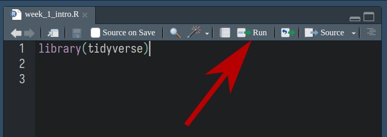
• Second is to use the keyboard shortcut Ctrl-Enter. This will also run the line of code that your cursor is on, and is the option I typically use.

When you do this, you’ll (hopefully) see a bunch of messages like this in the console down below:

These messages are nothing to worry about, they’re just telling you what new tools you have because you loaded the Tidyverse package.

Downloading data

For this lesson, we’re going to look at the names of horses in Switzerland, A very important topic that affects all of our lives. The data set can be found at:

https://tierstatistik.identitas.ch/en/equids-topNamesFemale.html

https://tierstatistik.identitas.ch/en/equids-topNamesMale.html

Making a new folder on your computer in RStudio

Before we download the data, we should make a new folder to put it in. This will keep our project organized, and make it easier to find things later.

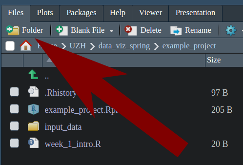
In the lower right hand corner, you’ll see a “Files” tab. This has a button that looks like a folder with a plus sign on it. Click this to make a new folder, and call it input_data.

Downloading files using `download.file()`

The first thing we need to do is download the data. We can do this with the download.file() function. This takes two arguments: the URL of the file you want to download, and the name of the file you want to save it as. They should be separated with a comma, and in quotes.

This is a function, a piece of code that does something. In this case, it downloads a file from the internet.

Please copy the code below and paste it into your new file.

Downloading directly from the web

If you’re using RStudio on your own computer, you have the option to do this manually.

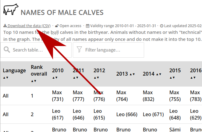
When we look at this data set, we can see that we have the option to “Download the data (CSV)”. Do that.

Now, find your downloaded file, and put it in the same folder as your project. I usually keep my raw, untouched data in a sub-folder called “input_data”, but you can organize your files however you like.

Importing data

The first thing we should always do with any data we get is to just to open it up and take a look. You should see it in your file screen, and if you click on it, you’ll have the option to View File, which just opens it as a text file in RStudio.

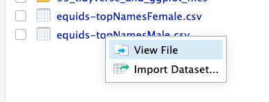
You can also do this in something like Notepad if you prefer. It will look similar to this:

Not very beautiful, but useful! Here are some things that we might notice:

1. The first line is some meta-information that we don’t need. We don’t want to import that.
2. This is in the form of a table. Each column of information is separated by a semicolon (;).
3. The second row is the names of each column of information. We should treat this row as a header.

Fortunately, RStudio has all the tools we need to help you do this. We can get started by opening the “Import Dataset” dialog.

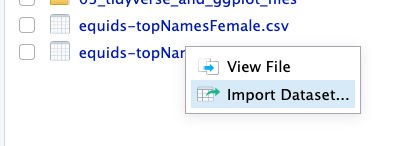
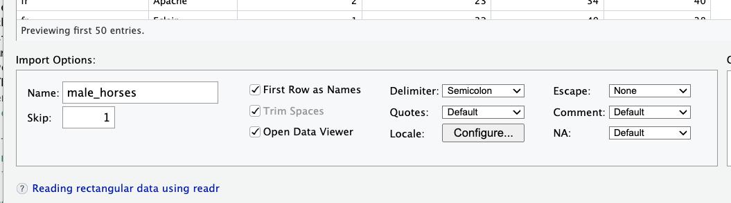
In the bottom left, you’ll see the import options. We’ll need to adjust some of them to make this work.

1. We should set Skip: to 1, to skip that first line of metadata.
2. The “Delimiter” is the thing that separates our data. For this dataset, we’ll use a semicolon.
3. Make sure that “First Row as Names” is checked. This sets the column names.
4. “equids_topNamesMale” will be an annoying name to type. Change the Name: to something more convenient.

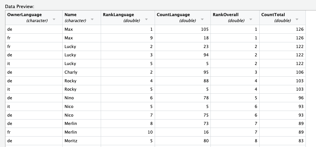
Your option box should look like this:

If you’ve done everything correctly, you should see that the columns have been cleanly separated, and each column has a name.

But don’t hit the import button! We want to focus on reproducibility, so we should make sure that our code runs without clicking these dialogues every time. Instead, copy the code from the code preview, and paste it into your source code.

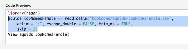
Do the same thing with the other horse data set. After this step, your code should look something like this:

Now, run this code. In the upper right hand panel on your screen, you should see that two new things have shown up, male_horses and female_horses.

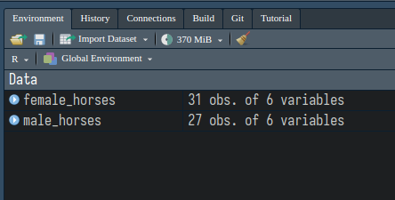
This means that the data is now living in R’s memory, and we can access it using that name.

Additionally, if you click on the name of the variable, you can see the data in a table format.

Data pipelines

But how to do things with this? This symbol will be your new best friend:

This is called a pipe, and because it moves data from one place to the next.

All this does is take the results of your last step, and pass it to your next function. This allows us to do many small steps at once, and split up our data pipelines into small, readable steps.

We combine these with specially-made functions to arrange and organize our data.

You’ll be typing this a lot, and it’s really handy to use a keyboard shortcut for the pipe. By default, it is something like Ctrl-Shift-M.

[!NOTE]

What if it says %>% instead of |>?

When you type Ctrl-Shift-M, you might get a different result, namely this: %>%.

To fix this, you can go to the go to the “Tools” > “Global Options” menu. Then open up the “Code” tab. Check the box that says “Use native pipe operator”. You can find more details in the installation chapter.

Seeing the start of some data with `head()`

The first of these special functions we’ll learn is head(), which just shows the first few lines of our data.

It’s useful for taking a look at really big datasets; let’s try it out with a pipe:

Counting rows with `count()`

Another useful function is count(), which gives the total number of rows, divided by the number of columns you select. For example, if I wanted to know the total number of names in each language, I could pipe |> the OwnerLanguage into count.

The output is always the input columns and n, which is the number of rows.

Filtering out only the stuff we want with `filter()`

This gives us a little preview of what we’re looking at, so new we can go ahead and search for the data that we want, by filtering out data that we don’t need.

One of the most important of these functions is filter(). Filtering only keeps the rows that we want, just like a coffee filter keeps only the liquid we want to drink, while getting rid of the gritty ground beans.

Let’s say we wanted to find out the most common name for a horse with a German-speaking owner. Having looked at our data’s head, we can see that the column OwnerLanguage will tell us this information. To keep only the German data, we could use a filter like this:

That’s great, but what if we only wanted the top 3 names? We could use a second filter, with one piping into the next.

Even better, but those maybe we don’t need those other columns in our final analysis, so we can just select the ones that we need.

Selecting only the columns we want with `select()`

Just like filter() filters out the rows that we want, select() can select only the columns that we want. We simply pass the names of the columns that we need, and only those will be taken.

In this example, we just want the top 3 horses, as well as the language count.

Great! But CountLanguage is kind of an awkward name. Can we rename it?

Giving columns better names with `rename()`

The rename function, as the name implies, renames columns. We can use it to make our data more readable.

Changing data with `mutate()`

Much cleaner. However, sometimes we want to change something inside the cell. We can use mutate() to make new columns with slightly changed data, or replace a column that we have, using a function.

Maybe we want to make the names uppercase, like we are yelling at our horse. We already know that you can use toupper to change some text, like so:

To apply this to our data, we can use the mutate(), like so:

We can even overwrite the original column with mutate, instead of making a new one:

Soon, we will combine this with the male dataset, but we need to remember if each of these names is for a mare or a stallion. We can simply mutate a new column with the sex of the horse.

Pretty clean, I’m happy with that!

Saving variables with `<-`

Until now, we’ve been doing things to our data, then just printing it out. Sometimes, we want to save our work so we can use it later. We can do this with the assignment operator, <-.

The assignment operator saves whatever we put in front of it to memory, so we can use it later. For example, if we just wanted to save our name, we could do this:

When we run this code, nothing will show up in the console. However, if we type my_name and run it, it will print out your name. You should also see it listed in the environment panel in the upper right hand corner.

In this case, we want to use the assignment operator to save our new data frame. We can call it german_mares. We put this at the beginning of the line, and then run the code.

Note that nothing shows up when you type this, because we haven’t told R to show it to us. If you’re feeling paranoid, just type the name of a variable and it will print.

[!NOTE]

What if I wanted to call it something else?

You can name your variables whatever you like, but there are some rules.

• You can’t have spaces in the name.
• You can’t start with a number.
• Capitalization matters, so my_name is different from My_Name.
• You can’t use special characters like !, @, #, $ or %.
• Two things can’t have the same name, so you can’t have two variables called my_name.

In addition, we have some general conventions in R:

• We use lowercase for variable names, and separate words with an underscore, like my_name.
• The name should be descriptive, so you know what it is later.

Combining data with `bind_rows()`

The mares are ready, but what about the stallions? With a little copy-paste, we can simply re-do the same process for the males:

Our next step is to combine the two datasets into one. We can do this with bind_rows(). It adds one dataset to another, vertically. We pass the second dataset as an argument, and it plops them one on top of another.

bind_cols()

A related function is bind_cols(), which adds one dataset to another, horizontally. This is useful when you have two datasets with the same number of rows, and you want to combine them into one dataset with more columns.

Here is an example of using bind_rows() and bind_cols() to combine some datasets:

First, I’m going to make some fake data, in this case a table with people’s names, ages and jobs.

Now I’m going to make another table with some other people’s names, ages and jobs.

if we want to put them together on top of each other, we use bind_rows(). Note that they have to have the same column names.

I can then assign them to a new variable, all_people. This saves it in our environment.

However, I not have some other information about these people, such as their height and weight. I want to add this to the all_people dataset.

I can do this with bind_cols(). Note that the two tables must have the same number of rows.

Check your knowledge

1. Find the location of the folder for the project you made. Hopefully you put it somewhere sensible like your “documents” folder.

2. Review how to use the following functions:

3. Know that <- does, and how this is different from printing to the console.

Homework: Cleaning a similar dataset

The dataset for cattle is arranged differently. Can you figure out how to produce the same final table for German cows?

The raw data can be found here:

https://tierstatistik.identitas.ch/en/cattle-NamesFemaleCalves.html

https://tierstatistik.identitas.ch/en/cattle-NamesMaleCalves.html

Hint: There are a lot of different years in this data set. We only need the current year.

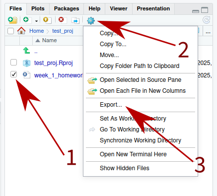
Please save your script as week_1_homework_(your_name).R and email it to me by Tuesday, February 25th.

If you’re using the web server, you’ll want to find the file in the lower right hand corner, check the box next to the file, then go to (gear symbol) > “Export …”. This will download the file to your computer.