Finding your own data sets
1 library(tidyverse)
Finding your own data sets
So far, we’ve been relying on some pretty simple example data, mainly from the Swiss government. This week, we’re going to look at how you can find your own data sets, so you can work on projects that are interesting to you.
Using national data portals
Just about every country has some sort of national data portal or statistical bureau that collects and publishes data. These are great places to find data, because the data is usually well-organized and reliable. A couple examples are:
- Canada: https://open.canada.ca/en
- Germany: https://www-genesis.destatis.de/genesis/online
- Taiwan: https://data.gov.tw/en
Classwork: Finding demographic data
-
Think of a place that you’re interested in (besides Switzerland, because we’ve done a lot of this already)
-
Find the website of the statistical bureau or data portal of that country.
-
Find a dataset that contains the following information:
- Population of each state / province / canton / region
- Something related to the economy (GDP, unemployment, etc.)
- Something related to health (life expectancy, infant mortality,
etc.)
- Something related to education (literacy rate, school enrollment,
etc.)
- Something related to the environment (CO2 emissions, forest cover,
etc.)
- Download the data and load it into R.
Effectively searching for data
When you’re looking for data, it’s important to use the right search terms. Here are a few tips:
-
Use the
filetype:operator to search for specific file types. For example, if you’re looking for CSV files using Google, you can search for filetype:csv canadian housing, and it will only return CSV files. -
Use the
site:operator to search within a specific website. For example, if you’re looking for data on the Swiss government’s website, you can search for site:admin.ch population. -
Use the
intitle:operator to search for specific words in the title of a page. For example, if you’re looking for data on the Swiss government’s website, you can search for intitle:migration site:admin.ch.
R Packages that supply data
There are a few R packages that can help you get data from various sources. Here are a few of the more useful ones:
Eurostat
Eurostat is the statistical office of the European Union. They collect
data on a wide range of topics, including agriculture, trade, and the
environment. You can access their data using the eurostat package,
which you might have to install seperately.
1 install.packages("eurostat")
1 library(eurostat)
This package has a search_eurostat function that you can use to search
for data sets. For example, if you’re interested in animal statistics,
you can search for “Animal”. This will return a data frame with the
results of the search, including codes for the data sets.
1 animal_stats <- search_eurostat("Animal")
2 animal_stats
# A tibble: 6 × 9 title code type last.update.of.data last.table.structure…¹ data.start <chr> <chr> <chr> <chr> <chr> <chr> 1 Animal popu… agr_… data… 27.03.2025 02.12.2024 1977 2 Animal hous… ef_a… data… 28.08.2024 28.08.2024 2010 3 Animal hous… ef_a… data… 16.07.2024 16.07.2024 2010 4 Animal hous… ef_a… data… 16.07.2024 16.07.2024 2010 5 Animal popu… agr_… data… 27.03.2025 02.12.2024 1977 6 Animal popu… agr_… data… 27.03.2025 02.12.2024 1977 # ℹ abbreviated name: ¹last.table.structure.change # ℹ 3 more variables: data.end <chr>, values <dbl>, hierarchy <dbl>
However, I’ve always found this to be a bit janky and not very useful. You might have better luck searching the website.
In either case, you just want to find the code for the data set you’re
interested in. Once you have that, you can use the get_eurostat
function to download the data.
1 animal_data <- get_eurostat("agr_r_animal")
2 animal_data
# A tibble: 30 × 7
...1 freq  animals unit   geo   TIME_PERIOD values
<dbl> <chr> <chr>   <chr>  <chr> <date>       <dbl>
1     1 A     A2000   THS_HD AT    1977-01-01   2547.
2     2 A     A2000   THS_HD AT    1978-01-01   2594.
3     3 A     A2000   THS_HD AT    1979-01-01   2548.
4     4 A     A2000   THS_HD AT    1980-01-01   2517.
5     5 A     A2000   THS_HD AT    1981-01-01   2530.
6     6 A     A2000   THS_HD AT    1982-01-01   2546.
7     7 A     A2000   THS_HD AT    1983-01-01   2633.
8     8 A     A2000   THS_HD AT    1984-01-01   2669.
9     9 A     A2000   THS_HD AT    1985-01-01   2651.
10    10 A     A2000   THS_HD AT    1986-01-01   2637.
# ℹ 20 more rows
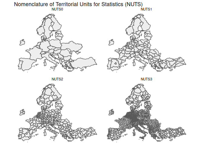
Eurostat often uses a geographical division called the NUTS (Nomenclature of Territorial Units for Statistics) system. This system divides countries into regions, which are then divided into smaller regions, and so on. The idea is to have a consistent way of dividing up countries into similar-sized areas for statistical purposes. Often, this doesn’t correspond to any administrative divisions, but it’s useful for comparing regions across countries.
World Bank Statistics
Next, we have the wbstats package, which allows you to access data
from the World Bank. This can give you a lot of economic data between
countries.
1 install.packages("wbstats")
1 library(wbstats)
Like Eurostat, the wb_search function allows you to search for data
sets
1 wb_search("electricity")
# A tibble: 127 × 3
indicator_id                   indicator                       indicator_desc
<chr>                          <chr>                           <chr>
1 1.1_ACCESS.ELECTRICITY.TOT     Access to electricity (% of to… Access to ele…
2 1.2_ACCESS.ELECTRICITY.RURAL   Access to electricity (% of ru… Access to ele…
3 1.3_ACCESS.ELECTRICITY.URBAN   Access to electricity (% of ur… Access to ele…
4 2.0.cov.Ele                    Coverage: Electricity           The coverage …
5 2.0.hoi.Ele                    HOI: Electricity                The Human Opp…
6 4.1.1_TOTAL.ELECTRICITY.OUTPUT Total electricity output (GWh)  Total electri…
7 4.1.2_REN.ELECTRICITY.OUTPUT   Renewable energy electricity o… Renewable ene…
8 4.1_SHARE.RE.IN.ELECTRICITY    Renewable electricity (% in to… Renewable ele…
9 9060000                        9060000:ACTUAL HOUSING, WATER,… <NA>
10 BM.GSR.TRAN.ZS                 Transport services (% of servi… Transport cov…
# ℹ 117 more rows
And like Eurostat, you can use the wb_data function to download the
data.
1 wb_data("4.1.1_TOTAL.ELECTRICITY.OUTPUT")
# A tibble: 30 × 10 ...1 iso2c iso3c country date 4.1.1_TOTAL.ELECTRICITY.OU…¹ unit obs_status <dbl> <chr> <chr> <chr> <dbl> <dbl> <lgl> <lgl> 1 1 AW ABW Aruba 1990 338 NA NA 2 2 AW ABW Aruba 1991 339 NA NA 3 3 AW ABW Aruba 1992 341 NA NA 4 4 AW ABW Aruba 1993 531 NA NA 5 5 AW ABW Aruba 1994 564 NA NA 6 6 AW ABW Aruba 1995 616 NA NA 7 7 AW ABW Aruba 1996 642 NA NA 8 8 AW ABW Aruba 1997 675 NA NA 9 9 AW ABW Aruba 1998 730 NA NA 10 10 AW ABW Aruba 1999 738. NA NA # ℹ 20 more rows # ℹ abbreviated name: ¹`4.1.1_TOTAL.ELECTRICITY.OUTPUT` # ℹ 2 more variables: footnote <lgl>, last_updated <date>
BFS data
If you’re going to be working frequently with Swiss data, you can use an R package built by the Swiss Federal Statistical Office (BFS) to access their data.
1 install.packages("BFS")
1 library(BFS)
This works essentially the same as the last two; you can search for data
sets using the bfs_get_catalog_data function, and download data using
the bfs_get_data function.
1 bfs_get_catalog_data(language = "en", extended_search = "university")
# A tibble: 6 × 6
title                 number_bfs language number_asset publication_date url_px
<chr>                 <chr>      <chr>    <chr>        <date>           <chr>
1 University of applie… px-x-1502… en       36454608     2026-03-24       https…
2 University of applie… px-x-1502… en       36454606     2026-03-24       https…
3 University students … px-x-1502… en       36454426     2026-03-24       https…
4 University students … px-x-1502… en       36454424     2026-03-24       https…
5 Businesses by diffic… px-x-0602… en       36412539     2026-02-26       https…
6 Businesses by diffic… px-x-0602… en       36412544     2026-02-26       https…
1 bfs_get_data(number_bfs = "px-x-1502040100_132", language = "en") |> write_csv("input_data/university_enrollment.csv")
# A tibble: 30 × 5
Year    `ISCED Field`     `Citizenship (category)` `Level of study`
<chr>   <chr>             <chr>                    <chr>
1 1990/91 Education science Switzerland              First university degree o…
2 1990/91 Education science Switzerland              Bachelor
3 1990/91 Education science Switzerland              Master
4 1990/91 Education science Switzerland              Doctorate
5 1990/91 Education science Switzerland              Further education, advanc…
6 1990/91 Education science Foreign country          First university degree o…
7 1990/91 Education science Foreign country          Bachelor
8 1990/91 Education science Foreign country          Master
9 1990/91 Education science Foreign country          Doctorate
10 1990/91 Education science Foreign country          Further education, advanc…
# ℹ 20 more rows
# ℹ 1 more variable: `University students` <dbl>
Web scraping
Our final method of acquiring data is the real wild west: web scraping.
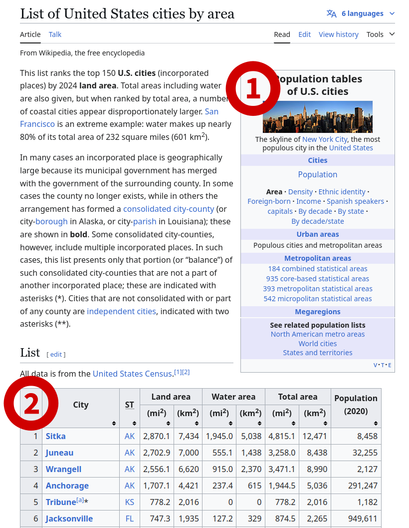
Extracting usable data from websites, is a really, really big topic, and one that we can’t really cover in depth in one lesson. However, we can do some basic web scraping that will get you pretty far. In this little bottled example, we’ll scrape a table from Wikipedia, in this case a list of US cities by area.
To do this, we’ll use the rvest package, which you might have to
install.
1 install.packages("rvest")
1 library(rvest)
Attaching package: 'rvest'
The following object is masked from 'package:readr':
guess_encoding
This gives us quite a few functions to download and parse HTML. We’ll
start by downloading the HTML of the page using the read_html
function.
1 html <- read_html("https://en.wikipedia.org/wiki/List_of_United_States_cities_by_area")
2 3 html
{html_document}
<html class="client-nojs vector-feature-language-in-header-enabled vector-feature-language-in-main-menu-disabled vector-feature-language-in-main-page-header-disabled vector-feature-page-tools-pinned-disabled vector-feature-toc-pinned-clientpref-1 vector-feature-main-menu-pinned-disabled vector-feature-limited-width-clientpref-1 vector-feature-limited-width-content-enabled vector-feature-custom-font-size-clientpref-1 vector-feature-appearance-pinned-clientpref-1 skin-theme-clientpref-day vector-sticky-header-enabled wp25eastereggs-enable-clientpref-1 vector-toc-available skin-theme-clientpref-thumb-standard" lang="en" dir="ltr">
[1] <head>\n<meta http-equiv="Content-Type" content="text/html; charset=UTF-8 ...
[2] <body class="skin--responsive skin-vector skin-vector-search-vue mediawik ...
This gives us the HTML of the page, just the code that makes up the website.
HTML is a markup language, which means it’s a way of describing the
structure of a document. It’s made up of tags, which are enclosed in
angle brackets. For example, <h1> is a tag that indicates a heading,
<h2> is a subheading, and so on.
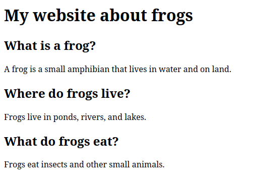
Here’s a simple example:
1 <!DOCTYPE html>
2 <html>
3 <head>
4 </head>
5 <body>
6 <!-- The h1 tag is a heading-1, which is usually the title of the page -->
7 <h1>My website about frogs</h1>
8
9 <!-- The h2 tag is a heading-2, which is a subheading, usually denoting a section -->
10 <h2>What is a frog?</h2>
11
12 <!-- The p tag is a paragraph, which is used for text -->
13 <p>A frog is a small amphibian that lives in water and on land.</p>
14
15 <!-- You can have multiple tags of any type -->
16 <h2>Where do frogs live?</h2>
17 <p>Frogs live in ponds, rivers, and lakes.</p>
18
19 <h2>What do frogs eat?</h2>
20 <p>Frogs eat insects and other small animals.</p>
21 </body>
22 </html>
When opened in a web browser, this would look like this:
We can now use the html_nodes function to extract specific parts of
the page. For example, to extract all the H1 tags, we can use the
following code:
1 html |>
2 html_nodes("h1")
{xml_nodeset (1)}
[1] <h1 id="firstHeading" class="firstHeading mw-first-heading"><span class=" ...
For H2 tags, we can use this code. To get all the text inside the tags,
we can use the html_text function.
Note that there are multiple H2 tags on the page, so we get a list of them.
1 html |>
2 html_nodes("h2") |>
3 html_text()
[1] "Contents"          "List"              "Gallery"
[4] "See also"          "Explanatory notes" "References"
We can also extract tables from the page. To do this, we can use the
html_nodes function with the table tag.
1 tables_on_page <- html |>
2 html_nodes("table")
3 4 tables_on_page
{xml_nodeset (2)}
[1] <table class="sidebar nomobile nowraplinks" role="navigation"><tbody>\n<t ...
[2] <table class="sortable wikitable sticky-header-multi static-row-numbers s ...
Because there are multiple tables on the page, we get a list of them. We can extract the second table, which is the one we’re interested in. You can go back to the website and count down to whatever table you want to extract, or just do it with trial-and-error.
The structure of this data is a little odd, because it’s a list of lists. We extract the second element of the list, which is the table we want.
1 cities_table <- tables_on_page[[2]]
2 cities_table
{html_node}
<table class="sortable wikitable sticky-header-multi static-row-numbers sort-under col1left col2center" style="text-align:right">
[1] <tbody>\n<tr>\n<th rowspan="2">City\n</th>\n<th rowspan="2">\n<abbr title ...
Finally, we can use the html_table function to convert this table into
a data frame.
1 cities_df <- cities_table |>
2 html_table()
3 4 cities_df
# A tibble: 151 × 9
City     ST    `Land area` `Land area` `Water area` `Water area` `Total area`
<chr>    <chr> <chr>       <chr>       <chr>        <chr>        <chr>
1 City     ST    (mi2)       (km2)       (mi2)        (km2)        (mi2)
2 Sitka    AK    2,870.2     7,434       1,904.3      4,932        4,774.5
3 Juneau   AK    2,702.9     7,000       555.1        1,438        3,258.0
4 Wrangell AK    2,556.1     6,620       915.0        2,370        3,471.1
5 Anchora… AK    1,706.8     4,421       237.7        616          1,944.5
6 Tribune… KS    778.2       2,016       0            0            778.2
7 Jackson… FL    747.3       1,935       127.1        329          874.5
8 Anacond… MT    736.7       1,908       4.7          12           741.4
9 Butte *  MT    715.8       1,854       0.6          1.6          716.3
10 Houston  TX    640.8       1,660       31.2         81           672.0
# ℹ 141 more rows
# ℹ 2 more variables: `Total area` <chr>, `Population(2020)` <chr>
That’s it! You’ve now scraped a table from Wikipedia. This is a very basic example, but you could use this basic concept to scrape data from any website that has tables on it.
Classwork: Scraping a table from the BBC
Here’s a link to the BBC’s election results page for the 2024 UK general election:
https://www.bbc.com/news/election/2024/uk/results
This page has a table with the results of the election. Your task is to scrape this table and load it into R as a data frame.
Your result should look something like this:
# A tibble: 34 × 3
Party                     `Vote share` `Change since 2019`
<chr>                     <chr>        <chr>
1 Labour                    33.7%        +1.6%
2 Conservative              23.7%        −19.9%
3 Reform UK                 14.3%        +12.3%
4 Liberal Democrat          12.2%        +0.7%
5 Green                     6.7%         +4.0%
6 Scottish National Party   2.5%         −1.4%
7 Plaid Cymru               0.7%         +0.2%
8 Sinn Fein                 0.7%         +0.1%
9 Workers Party of Britain  0.7%         +0.7%
10 Democratic Unionist Party 0.6%         −0.2%
# ℹ 24 more rows
Some web scraping tips
- Be polite: Don’t scrape websites too often, and don’t scrape them too fast. This can overload the server and get you banned.
- Save the data: Once you’ve scraped the data, save it to a file. This way, you don’t have to scrape the website again. Websites can change, and you might not get the same data if you scrape it again.
- Check the terms of service: Some websites don’t allow scraping. If you’re doing something that isn’t allowed, be extra careful. If you’re selling the data, it could get you in some real legal trouble.
Next steps with web scraping
If you’d like to keep using R, the book “R for Data Science” has a great chapter on web scraping. You can find it here: https://r4ds.hadley.nz/webscraping.html
However, R is pretty limited when it comes to web scraping. If you’re interested in doing more complicated things, I’d recommend learning Python or Go.