Tables and statistics
1 install.packages("gt")
2 install.packages("gtsummary")
3 install.packages("broom")
4 install.packages("broom.helpers")
5 install.packages("webshot2")
6 install.packages("report")
1 library(tidyverse)
2 library(wbstats)
3 library(countrycode)
4 library(gt)
5 library(gtsummary)
6 library(report)
This week, we’re actually going to be social scientists, and run a study from start to finish: We’ll generate hypotheses, gather data, run a regression model, and write up the results.
Understanding linear regression
This is not a statistics class, but for this class we’re going to dive into it a little bit, running a linear regression, and understanding what it means.
Formulating a hypothesis
I study the news media, and want to understand what factors might influence newspaper circulation. Thinking for a few seconds, I believe that a richer countries have more newspapers, and that people in those countries read more newspapers.
Of course, we have to be very careful not to talk about causation here. We can say that there is a correlation between GDP per capita and newspaper circulation, but we can’t say that one causes the other. Maybe richer countries have more newspapers, or reading a newspaper makes you richer. Or maybe both are caused by a third factor, like education or literacy.
We first write out a hypothesis, which is a statement that we can test with data. In this case, I might say:
Hypothesis 1: Countries with a higher GDP per capita have a higher newspaper circulation.
Gathering our data
Ok, so we have a hypothesis. Now we need to gather some data to test it. We need two things: Newspaper circulation data, and GDP per capita data.
Newspaper circulation
We can get newspaper circulation data from the UN data website. The data is in a zip file, so we need to download it and unzip it.
1 download.file("https://data.un.org/Handlers/DownloadHandler.ashx?DataFilter=series:C_N_CDN&DataMartId=UNESCO&Format=csv&c=2,3,5,7,9,10&s=ref_area_name:asc,time_period:desc", "input_data/un_data.zip")
2 3 unzip("input_data/un_data.zip", exdir = "input_data/un_data")
1 # Daily newspapers: Total average circulation per 1,000 inhabitants2 newspaper_circulation <- 3 read_csv("input_data/un_data/UNdata_Export_20250514_074704100.csv") |>
4 group_by(`Reference Area`) |>
5 filter(`Time Period` == max(`Time Period`)) |>
6 mutate(iso3c = countrycode(`Reference Area`, "country.name", "iso3c")) |>
7 mutate(un_region = countrycode(iso3c, "iso3c", "un.region.name")) |>
8 select(iso3c, un_region, `Reference Area`, `Observation Value`) |>
9 rename(10 country = `Reference Area`,
11 circulation = `Observation Value`12 ) |>
13 ungroup()
14 15 newspaper_circulation
# A tibble: 183 × 4
iso3c un_region country     circulation
<chr> <chr>     <chr>             <dbl>
1 AFG   Asia      Afghanistan        5.96
2 ALB   Europe    Albania           24.4
3 DZA   Africa    Algeria           37.6
4 AGO   Africa    Angola             2.24
5 ARG   Americas  Argentina         35.5
6 ARM   Asia      Armenia            7.60
7 ABW   Americas  Aruba            842.
8 AUS   Oceania   Australia        155.
9 AUT   Europe    Austria          311.
10 AZE   Asia      Azerbaijan        16.1
# ℹ 173 more rows
GDP per capita
We also need GDP per capita data. We can get this from the World Bank. The World Bank has a nice API discussed in chapter 4 that we can use to get the data.
1 wb_search("gdp per capita")
1 gdp_per_capita <- wb_data(indicator = "NY.GDP.PCAP.CD", start_date = 2019, end_date = 2019)
2 3 gdp_per_capita <- 4 gdp_per_capita |>
5 select(iso3c, NY.GDP.PCAP.CD) |>
6 rename(7 gdp_per_capita = NY.GDP.PCAP.CD8 ) |>
9 mutate(10 gdp_per_capita = gdp_per_capita / 1000
11 )Finally, we use the iso3c code to join the two data frames together. We drop the NA values here, because we don’t want to include countries that don’t have data for both variables. This results in fewer countries in our study than before, but we can just add that to the limitations section, don’t worry.
1 regression_df <- 2 newspaper_circulation |>
3 left_join(gdp_per_capita, by = c("iso3c" = "iso3c")) |>
4 drop_na()
Running a linear regression with `lm()`
Now, we want to test our hypothesis. We can do this with a linear
regression model. Remember way back when, we used the geom_smooth()
function to fit a linear regression line to our scatter plot? This is
the same thing, but we can get more information out of it.
Code
1 regression_df |>
2 ggplot(aes(x = gdp_per_capita, y = circulation)) +
3 geom_point() +
4 geom_smooth(method = "lm") +
5 theme_minimal() +
6 labs(7 x = "GDP per capita",
8 y = "Newspaper circulation (per 1,000 inhabitants)",
9 title = "Newspaper circulation vs GDP per capita"
10 )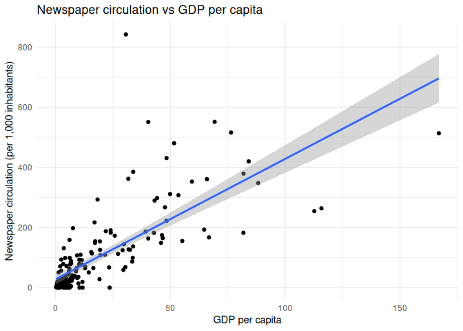
The lm() function in R is used to fit linear models, and it takes a
formula as its first argument. The formula is of the form
y ~ x1 + x2 + ..., where y is the dependent variable, and x1,
x2, etc. are the independent variables. In this case, we have only one
independent variable, gdp_per_capita, so the formula is
circulation ~ gdp_per_capita.
When we run the lm() function, it returns an object that contains the
results of the regression. We can use the summary() function to get a
summary of the results.
1 univariate_regression_model <- lm(circulation ~ gdp_per_capita, data = regression_df)
2 3 univariate_regression_model |>
4 summary()
Call:
lm(formula = circulation ~ gdp_per_capita, data = regression_df)
Residuals:
Min      1Q  Median      3Q     Max
-227.66  -31.52  -23.60   20.75  691.91
Coefficients:
Estimate Std. Error t value Pr(>|t|)
(Intercept)     27.7379     8.3909   3.306  0.00115 **
gdp_per_capita   4.0051     0.2714  14.758  < 2e-16 ***
---
Signif. codes:  0 '***' 0.001 '**' 0.01 '*' 0.05 '.' 0.1 ' ' 1
Residual standard error: 90.62 on 174 degrees of freedom
Multiple R-squared:  0.5559,    Adjusted R-squared:  0.5533
F-statistic: 217.8 on 1 and 174 DF,  p-value: < 2.2e-16
Reading a regression table
What are we looking at here? When an outsider is looking at your regression table, they will focus on a few things in particular:
- The
Coefficientstable shows the estimated coefficients for each independent variable. In this case, we have one independent
variable, `gdp_per_capita`, and its estimated coefficient is 4.0126.
This means that for every 1,000 USD increase in GDP per capita,
newspaper circulation increases by 0.4 newspapers per 1,000
inhabitants.
Pr(>|t|)columns shows the p-value for each coefficient. The p-value tells us whether the coefficient is statistically
significant. In this case, the p-value for `gdp_per_capita` is less
than 2e-16, or 0.0000000000000002, which means that it is very
statistically significant. However, p-values are very complicated
and often misleading, and the more you read about them, the more you
will understand that they are not the end of the story.
- The p-value is emphasized by some little stars. The stars are a shorthand for the p-value, and they tell you how statistically
significant the coefficient is. One star means that the p-value is
less than 0.05, two stars mean that it is less than 0.01, and three
stars mean that it is less than 0.001. In this case, we have three
stars, which means that the coefficient is very statistically
significant. Don’t worship the stars, though! As we’ll see, this is
very easy to manipulate.
- The
Multiple R-squaredvalue is a measure of how well the model fits the data. It is the proportion of variance in the dependent
variable that is explained by the independent variable(s). In this
case, the `Multiple R-squared` value is 0.5568, which means that
about 55.7% of the variance in newspaper circulation is explained by
GDP per capita.
The rest of this stuff you should learn from a statistics class. Just know that when reviewers are looking at your scientific paper, these are the things that they’ll zoom in on.
Adding a third variable: Literacy
Ok, so we’ve tested our hypothesis, and we found that there is a statistically significant relationship between GDP per capita and newspaper circulation. But we also know that there are other factors that might influence newspaper circulation, like literacy.
Countries with people that know how to read and write are more likely to have newspapers, and people that can read and write are more likely to read newspapers. So we want to add literacy as a third variable to our model.
First, we need to formulate a new hypothesis:
Hypothesis 2: Countries with a higher literacy rate have a higher newspaper circulation.
Then we need to get the data. We can get literacy data from the World
Bank, just like we did with GDP per capita. The indicator we want is
SE.ADT.LITR.ZS, which is the literacy rate for people aged 15 and
older.
1 wb_search("literacy")
We get the data through our API, and clean it up a little bit.
1 literacy_rate <- wb_data(indicator = "SE.ADT.LITR.ZS")
2 3 literacy_rate <- literacy_rate |>
4 drop_na( SE.ADT.LITR.ZS) |>
5 group_by(iso3c) |>
6 filter(date == max(date)) |>
7 select(iso3c, SE.ADT.LITR.ZS) |>
8 rename(9 literacy_rate = SE.ADT.LITR.ZS10 ) |>
11 ungroup()
We then join it back into our main data frame.We should be pros at this by now.
1 regression_df <-2 regression_df |>
3 left_join(literacy_rate, by = c("iso3c" = "iso3c")) |>
4 drop_na()
5 6 regression_df
# A tibble: 147 × 6
iso3c un_region country     circulation gdp_per_capita literacy_rate
<chr> <chr>     <chr>             <dbl>          <dbl>         <dbl>
1 AFG   Asia      Afghanistan        5.96          0.497          37.3
2 ALB   Europe    Albania           24.4           6.07           97.7
3 DZA   Africa    Algeria           37.6           4.47           75.1
4 AGO   Africa    Angola             2.24          2.49           66.2
5 ARG   Americas  Argentina         35.5           9.96           99.1
6 ARM   Asia      Armenia            7.60          4.60           99.8
7 ABW   Americas  Aruba            842.           30.6            96.8
8 AZE   Asia      Azerbaijan        16.1           4.81           99.8
9 BHR   Asia      Bahrain          112.           27.3            97.8
10 BGD   Asia      Bangladesh         8.67          2.13           79
# ℹ 137 more rows
Now, let’s take a look at a univariate regression model with literacy rate as the only independent variable.
1 regression_df |>
2 lm(formula = circulation ~ literacy_rate) |>
3 summary()
Call:
lm(formula = circulation ~ literacy_rate, data = regression_df)
Residuals:
Min      1Q  Median      3Q     Max
-100.69  -50.73  -20.57   20.88  746.47
Coefficients:
Estimate Std. Error t value Pr(>|t|)
(Intercept)   -132.7952    40.3086  -3.294  0.00124 **
literacy_rate    2.3623     0.4644   5.087 1.11e-06 ***
---
Signif. codes:  0 '***' 0.001 '**' 0.01 '*' 0.05 '.' 0.1 ' ' 1
Residual standard error: 97.06 on 145 degrees of freedom
Multiple R-squared:  0.1514,    Adjusted R-squared:  0.1456
F-statistic: 25.88 on 1 and 145 DF,  p-value: 1.109e-06
Hell yeah! We have a statistically significant relationship between literacy rate and newspaper circulation.
But what happens when we make a multivariate regression model, with both GDP per capita and literacy rate as independent variables?
1 regression_df |>
2 lm(formula = circulation ~ gdp_per_capita + literacy_rate) |>
3 summary()
Call:
lm(formula = circulation ~ gdp_per_capita + literacy_rate, data = regression_df)
Residuals:
Min      1Q  Median      3Q     Max
-166.05  -25.75  -10.83   12.61  674.93
Coefficients:
Estimate Std. Error t value Pr(>|t|)
(Intercept)    -41.6163    32.3590  -1.286   0.2005
gdp_per_capita   4.5592     0.4552  10.016   <2e-16 ***
literacy_rate    0.7164     0.3937   1.820   0.0709 .
---
Signif. codes:  0 '***' 0.001 '**' 0.01 '*' 0.05 '.' 0.1 ' ' 1
Residual standard error: 74.77 on 144 degrees of freedom
Multiple R-squared:  0.4999,    Adjusted R-squared:  0.4929
F-statistic: 71.97 on 2 and 144 DF,  p-value: < 2.2e-16
Noooooo! Literacy rate is no longer statistically significant. Because GDP per capita and literacy rate are correlated, the model is telling us that GDP per capita is a better predictor of newspaper circulation than literacy rate. This is called multicollinearity, and it can be a problem in regression models.
Sometimes, the opposite can happen, as well, where a variable that is not statistically significant in a univariate model becomes significant in a multivariate model.
Because papers that include statistically significant results are more likely to be published, it’s a common temptation to just keep adding variables to your model until you get a statistically significant result. This is called p-hacking.
To avoid this, you should always start with a theoretical model, and then test it with data. Even better is to pre-register your hypotheses and methods before you collect your data.
Adding a categorical predictor
We’re not limited to just continuous variables in our regression model. We can also add categorical variables, like the UN region of a country.
If we look at the regression_df data frame, we can see that we have a
variable called un_region. We can use this as a categorical predictor
in our regression model.
Code
1 regression_df |>
2 ggplot(aes(y = un_region, x = circulation)) +
3 geom_boxplot() +
4 theme_minimal() +
5 labs(6 x = "Newspaper circulation per 1,000 inhabitants",
7 y = "UN subregion",
8 title = "Newspaper circulation by UN region"
9 )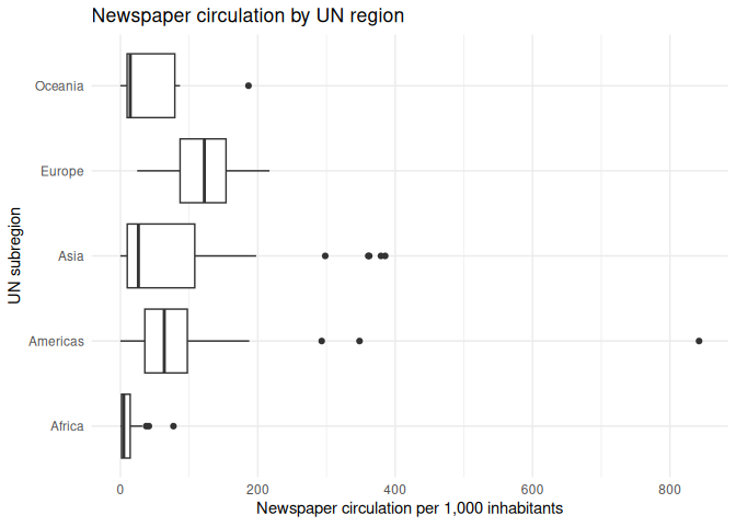
1 regression_df |>
2 lm(formula = circulation ~ un_region) |>
3 summary()
Call:
lm(formula = circulation ~ un_region, data = regression_df)
Residuals:
Min      1Q  Median      3Q     Max
-105.15  -54.11   -9.56   12.61  737.25
Coefficients:
Estimate Std. Error t value Pr(>|t|)
(Intercept)          11.16      14.22   0.785 0.433700
un_regionAmericas    93.98      22.78   4.125 6.27e-05 ***
un_regionAsia        71.03      20.57   3.453 0.000732 ***
un_regionEurope     110.25      26.03   4.236 4.07e-05 ***
un_regionOceania     42.92      39.49   1.087 0.279016
---
Signif. codes:  0 '***' 0.001 '**' 0.01 '*' 0.05 '.' 0.1 ' ' 1
Residual standard error: 97.48 on 142 degrees of freedom
Multiple R-squared:  0.1617,    Adjusted R-squared:  0.1381
F-statistic: 6.847 on 4 and 142 DF,  p-value: 4.547e-05
From this, we can see that there are some differences in newspaper circulation by UN region. However, we can also (annoyingly) notice that one of the UN’s five regions is missing. What’s going on?
The first region is always the reference category, and the other regions are compared to it. This means that the coefficients for the other regions tell us how much higher or lower newspaper circulation is in those regions compared to it.
Because lm() always chooses the first category as the reference
category, we can change the reference category by reordering the levels
of the factor. For example, but putting the Americas first, we can use
that as a baseline.
1 regression_df |>
2 mutate(un_region = fct_relevel(un_region, "Americas")) |>
3 lm(formula = circulation ~ un_region) |>
4 summary()
Call:
lm(formula = circulation ~ un_region, data = mutate(regression_df,
un_region = fct_relevel(un_region, "Americas")))
Residuals:
Min      1Q  Median      3Q     Max
-105.15  -54.11   -9.56   12.61  737.25
Coefficients:
Estimate Std. Error t value Pr(>|t|)
(Intercept)        105.15      17.80   5.908 2.45e-08 ***
un_regionAfrica    -93.98      22.78  -4.125 6.27e-05 ***
un_regionAsia      -22.96      23.19  -0.990    0.324
un_regionEurope     16.27      28.14   0.578    0.564
un_regionOceania   -51.06      40.92  -1.248    0.214
---
Signif. codes:  0 '***' 0.001 '**' 0.01 '*' 0.05 '.' 0.1 ' ' 1
Residual standard error: 97.48 on 142 degrees of freedom
Multiple R-squared:  0.1617,    Adjusted R-squared:  0.1381
F-statistic: 6.847 on 4 and 142 DF,  p-value: 4.547e-05
Note that comparing from a different baseline can affect the significance levels, and this is another way that unethical researchers can hack their results.
Creating a multivariate model
Last, we can create a multivariate model with all of our independent variables. This model will take into account the relationship of GDP per capita, literacy rate, and UN region with newspaper circulation.
1 regression_df |>
2 lm(formula = circulation ~ gdp_per_capita + literacy_rate + un_region) |>
3 summary()
Call:
lm(formula = circulation ~ gdp_per_capita + literacy_rate + un_region,
data = regression_df)
Residuals:
Min      1Q  Median      3Q     Max
-151.00  -26.44   -2.81    6.28  655.18
Coefficients:
Estimate Std. Error t value Pr(>|t|)
(Intercept)       -15.8308    35.4186  -0.447   0.6556
gdp_per_capita      4.5261     0.4570   9.904   <2e-16 ***
literacy_rate       0.2308     0.4979   0.463   0.6437
un_regionAmericas  41.9910    21.0924   1.991   0.0484 *
un_regionAsia       8.8372    19.3596   0.456   0.6488
un_regionEurope    38.1067    24.6918   1.543   0.1250
un_regionOceania   -9.6871    31.9515  -0.303   0.7622
---
Signif. codes:  0 '***' 0.001 '**' 0.01 '*' 0.05 '.' 0.1 ' ' 1
Residual standard error: 74.02 on 140 degrees of freedom
Multiple R-squared:  0.5235,    Adjusted R-squared:  0.5031
F-statistic: 25.64 on 6 and 140 DF,  p-value: < 2.2e-16
Great! Let’s practice this a little.
Classwork: Make and test some hypotheses
- Think up up with 2 more indicators that you think might be related to a country’s newspaper circulation, and write down a hypothesis
for each one.
- Download the data from any source you like.
- Join the data into your main
regression_dfdata frame. - Test them with a bivariate regression model (just the dependent variable and one independent variable).
- Test them with a multivariate regression model (the dependent variable and all the independent variables).
- Save this model to your environment.
Here’s an example:
- I think that old people read more newspapers, so the median age of a country might be related to newspaper circulation. I formulate this
as a hypothesis:
Hypothesis 3: “Countries with a higher median age have a higher newspaper circulation.”
- I found some data on the UN website
about the median age of a country. I have to download it manually:
Code
1 download.file("http://data.un.org/Handlers/DownloadHandler.ashx?DataFilter=MEASURE_CODE:WHS9_88&DataMartId=WHO&Format=csv&c=2,4,8&s=_crEngNameOrderBy:asc,_timeEngNameOrderBy:desc", "input_data/un_data_age.zip")
2 3 unzip("input_data/un_data_age.zip", exdir = "input_data/un_data_age")
- I can then read it in with
read_csv()and clean it up, then join it to my main data frame.
Code
1 median_age <- read_csv("input_data/un_data_age/UNdata_Export_20250514_085133171.csv")
2 3 median_age <- median_age |>
4 mutate(iso3c = countrycode(`Country or Area`, "country.name", "iso3c")) |>
5 select(iso3c, Value) |>
6 rename(median_age = Value)
Code
1 regression_df <- 2 regression_df |>
3 left_join(median_age, by = c("iso3c" = "iso3c")) |>
4 drop_na()
- I can then test it first with a bivariate regression model.
Code
1 lm(circulation ~ median_age, data = regression_df) |>
2 summary()
- And then with a multivariate regression model.
Code
1 multivariate_model <- 2 lm(circulation ~ gdp_per_capita + literacy_rate + median_age + un_region, data = regression_df)
3 4 multivariate_model |>
5 summary()
Call:
lm(formula = circulation ~ gdp_per_capita + literacy_rate + median_age +
un_region, data = regression_df)
Residuals:
Min       1Q   Median       3Q      Max
-119.176  -25.830    0.531   11.713  216.060
Coefficients:
Estimate Std. Error t value Pr(>|t|)
(Intercept)       -54.9109    25.9571  -2.115  0.03628 *
gdp_per_capita      3.7149     0.4408   8.428  5.5e-14 ***
literacy_rate      -0.2341     0.3496  -0.670  0.50424
median_age          3.6764     1.1698   3.143  0.00207 **
un_regionAmericas  12.9709    14.1225   0.918  0.36007
un_regionAsia      -0.5590    13.0937  -0.043  0.96601
un_regionEurope   -10.9146    23.0490  -0.474  0.63662
un_regionOceania   12.9814    25.0019   0.519  0.60449
---
Signif. codes:  0 '***' 0.001 '**' 0.01 '*' 0.05 '.' 0.1 ' ' 1
Residual standard error: 46.74 on 131 degrees of freedom
Multiple R-squared:  0.6397,    Adjusted R-squared:  0.6204
F-statistic: 33.22 on 7 and 131 DF,  p-value: < 2.2e-16
That’s science, baby! Send it off to Nature and buy some Prosecco for the apero.
Making good-looking tables
But wait, you might say, do I have to copy and paste all this stuff into a Word document? No, The reason I’ve taught you this was to give you some shortcuts to make your life easier.
A good scientific paper has good-looking tables, and they often follow the same basic structure: A table of summary statistics of all the variables going into the model, a table of regression results, and some stuff in the appendix for more detailed explanations.
Table 1: Summary statistics
First, we need to create a table of summary statistics for all the variables in our model. This is a good way to show the reader what the data looks like, and it can help them understand the results of the regression. This is good to have, because it keeps you from hiding some bad, weird data in your model.
the library gtsummary has a function called tbl_summary() that makes
this easy. It takes a data frame as its first argument, and it will
automatically calculate the summary statistics for all the variables in
the data frame.
We need to tell it which variables we want to include in the table. Because each line of the table is a different country, we want to exclude those from the results. Do this for all the variables in your model.
1 regression_df |>
2 tbl_summary(include = c(
3 "circulation",
4 "gdp_per_capita",
5 "literacy_rate",
6 "median_age",
7 "un_region"8 ))
| Characteristic | N = 1391 |
|---|---|
| circulation | 26 (6, 80) |
| GDP per capita (current US$) | 5 (2, 10) |
| Literacy rate, adult total (% of people ages 15 and above) | 92 (76, 98) |
| median_age | 26 (20, 31) |
| un_region | |
| Africa | 47 (34%) |
| Americas | 27 (19%) |
| Asia | 41 (29%) |
| Europe | 20 (14%) |
| Oceania | 4 (2.9%) |
| 1 Median (Q1, Q3); n (%) | |
We also have some options to customize the table. We can change the labels of the variables, and we can change the number of decimal places for the continuous variables.
I don’t expect you to memorize all the options, but you can look them up in the documentation when you need it.
1 regression_df |>
2 tbl_summary(include = c(
3 "circulation",
4 "gdp_per_capita",
5 "literacy_rate",
6 "median_age",
7 "un_region"8 ),
9 label = list(
10 circulation ~ "Newspaper circulation (per 1,000 inhabitants)",
11 gdp_per_capita ~ "GDP per capita (in USD)",
12 literacy_rate ~ "Literacy rate (%)",
13 median_age ~ "Median age (years)",
14 un_region ~ "UN region"
15 ),
16 digits = all_continuous() ~ 2,
17 )| Characteristic | N = 1391 |
|---|---|
| Newspaper circulation (per 1,000 inhabitants) | 26.17 (5.77, 80.15) |
| GDP per capita (in USD) | 4.60 (1.77, 10.46) |
| Literacy rate (%) | 92.01 (75.64, 97.68) |
| Median age (years) | 25.70 (19.62, 31.12) |
| UN region | |
| Africa | 47 (34%) |
| Americas | 27 (19%) |
| Asia | 41 (29%) |
| Europe | 20 (14%) |
| Oceania | 4 (2.9%) |
| 1 Median (Q1, Q3); n (%) | |
By default, tbl_summary() will show the median, first and third
quartiles for continuous variables, and the number of observations and
percentage for categorical variables. We can change this with the
statistic argument.
1 regression_df |>
2 tbl_summary(include = c(
3 "circulation",
4 "gdp_per_capita",
5 "literacy_rate",
6 "median_age",
7 "un_region"8 ),
9 label = list(
10 circulation ~ "Newspaper circulation (per 1,000 inhabitants)",
11 gdp_per_capita ~ "GDP per capita (in USD)",
12 literacy_rate ~ "Literacy rate (%)",
13 median_age ~ "Median age (years)",
14 un_region ~ "UN region"
15 ),
16 statistic = list(
17 all_continuous() ~ "{mean} ({sd})",
18 all_categorical() ~ "{n} / {N} ({p}%)"
19 ),
20 digits = all_continuous() ~ 2,
21 )| Characteristic | N = 1391 |
|---|---|
| Newspaper circulation (per 1,000 inhabitants) | 57.84 (75.87) |
| GDP per capita (in USD) | 9.07 (11.72) |
| Literacy rate (%) | 84.40 (17.55) |
| Median age (years) | 26.57 (7.86) |
| UN region | |
| Africa | 47 / 139 (34%) |
| Americas | 27 / 139 (19%) |
| Asia | 41 / 139 (29%) |
| Europe | 20 / 139 (14%) |
| Oceania | 4 / 139 (2.9%) |
| 1 Mean (SD); n / N (%) | |
Finally, we can use the as_gt() function to convert the table to a
gt object, which is the underlying package for making our tables. We
can then use the tab_header() function to add a title to the table.
You can do a lot more to customize the table, but I don’t want to overwhelm you with options. You can look at the gt documentation for more information.
We also save it to a variable here.
1 summary_stats_table <- regression_df |>
2 tbl_summary(include = c(
3 "circulation",
4 "gdp_per_capita",
5 "literacy_rate",
6 "median_age",
7 "un_region"8 ),
9 label = list(
10 circulation ~ "Newspaper circulation (per 1,000 inhabitants)",
11 gdp_per_capita ~ "GDP per capita (in USD)",
12 literacy_rate ~ "Literacy rate (%)",
13 median_age ~ "Median age (years)",
14 un_region ~ "UN region"
15 ),
16 statistic = list(
17 all_continuous() ~ "{mean} ({sd})",
18 all_categorical() ~ "{n} / {N} ({p}%)"
19 ),
20 digits = all_continuous() ~ 2,
21 ) |>
22 as_gt() |>
23 tab_header(24 title = "Summary statistics for newspaper circulation and its predictors"
25 )Finally, we can save the table to a Word document. If you’re not a fan of Word (I’m sure not), you can also save it to a PDF, HTML, LaTeX, or png file. The world is your oyster.
1 summary_stats_table |>
2 gtsave("summary_stats_table.docx")
Table 2: Regression results
Now we want to create a table of the regression results. We can use the
tbl_regression() function from the gtsummary package to do this. It
takes a model object as its first argument, and it will automatically
create a table of the regression results.
I’ve added the following options to the table:
- Just like before, we can customize the table labels with the
labelargument. - We can make significant p-values bold with the
bold_p()function. This is a good way to draw attention to the most important results
in the table.
- We can make the labels bold with the
bold_labels()function. - We can italicize the levels of the categorical variables with the
italicize_levels()function. - We can add a source note to the table with the
add_glance_source_note()function. This contains all the other
information about the model, like the R-squared value and the number
of observations.
- We can use the
as_gt()function to convert the table to agtobject, and add a title with thetab_header()function.
When you’re doing this for real, you should look at the documentation and see what you can do.
1 regression_table <- multivariate_model |>
2 tbl_regression(3 label = list(
4 gdp_per_capita ~ "GDP per capita (thousands of USD)",
5 literacy_rate ~ "Literacy rate (%)",
6 median_age ~ "Median age (years)",
7 un_region ~ "UN region"
8 )9 ) |>
10 bold_p(t = 0.05) |>
11 bold_labels() |>
12 italicize_levels() |>
13 add_glance_source_note() |>
14 as_gt() |>
15 tab_header(16 title = "Regression results for newspaper circulation and its predictors"
17 )18 19 regression_table
| Regression results for newspaper circulation and its predictors | |||
|---|---|---|---|
| Characteristic | Beta | 95% CI | p-value |
| GDP per capita (thousands of USD) | 3.7 | 2.8, 4.6 | <0.001 |
| Literacy rate (%) | -0.23 | -0.93, 0.46 | 0.5 |
| Median age (years) | 3.7 | 1.4, 6.0 | 0.002 |
| UN region | |||
| Africa | — | — | |
| Americas | 13 | -15, 41 | 0.4 |
| Asia | -0.56 | -26, 25 | >0.9 |
| Europe | -11 | -57, 35 | 0.6 |
| Oceania | 13 | -36, 62 | 0.6 |
| Abbreviation: CI = Confidence Interval | |||
| R² = 0.640; Adjusted R² = 0.620; Sigma = 46.7; Statistic = 33.2; p-value = <0.001; df = 7; Log-likelihood = -728; AIC = 1,473; BIC = 1,499; Deviance = 286,231; Residual df = 131; No. Obs. = 139 | |||
Table 3: Miscellaneous Data
Great, you’ve added these to your paper, submitted it, and moved on with your life. A few months later, reviewer no. 2 comes back and says that they want to see the full data set added to the appendix.
You can do this with the gt() function, which takes a data frame as
its first argument. If you have too much data for one page, you can use
the gt_split() function to split the table into multiple pages. Handy!
1 regression_df |>
2 gt() |>
3 tab_header(4 title = "Newspaper circulation and its predictors (Full data)"
5 ) |>
6 gt_split(row_every_n = 30) |>
7 gtsave("appendix_1.docx")
Automating your results section with `report()`
That handled my tables, but what about the text? I don’t want to have to write all that stuff out by hand. Luckily, I have a solution to that too: the report package.
The report() function takes a model object as its first argument, and
it will automatically create a report of the results. It will include
the coefficients, p-values, and confidence intervals for each
independent variable, as well as the R-squared value for the model. Just
take this, and re-word it a little bit so it sounds less robotic, and
you have half of your results section written up.
1 report(multivariate_model)
We fitted a linear model (estimated using OLS) to predict circulation with
gdp_per_capita, literacy_rate, median_age and un_region (formula: circulation ~
gdp_per_capita + literacy_rate + median_age + un_region). The model explains a
statistically significant and substantial proportion of variance (R2 = 0.64,
F(7, 131) = 33.22, p < .001, adj. R2 = 0.62). The model's intercept,
corresponding to gdp_per_capita = 0, literacy_rate = 0, median_age = 0 and
un_region = Africa, is at -54.91 (95% CI [-106.26, -3.56], t(131) = -2.12, p =
0.036). Within this model:
- The effect of gdp per capita is statistically significant and positive (beta
= 3.71, 95% CI [2.84, 4.59], t(131) = 8.43, p < .001; Std. beta = 0.57, 95% CI
[0.44, 0.71])
- The effect of literacy rate is statistically non-significant and negative
(beta = -0.23, 95% CI [-0.93, 0.46], t(131) = -0.67, p = 0.504; Std. beta =
-0.05, 95% CI [-0.21, 0.11])
- The effect of median age is statistically significant and positive (beta =
3.68, 95% CI [1.36, 5.99], t(131) = 3.14, p = 0.002; Std. beta = 0.38, 95% CI
[0.14, 0.62])
- The effect of un region [Americas] is statistically non-significant and
positive (beta = 12.97, 95% CI [-14.97, 40.91], t(131) = 0.92, p = 0.360; Std.
beta = 0.17, 95% CI [-0.20, 0.54])
- The effect of un region [Asia] is statistically non-significant and negative
(beta = -0.56, 95% CI [-26.46, 25.34], t(131) = -0.04, p = 0.966; Std. beta =
-7.37e-03, 95% CI [-0.35, 0.33])
- The effect of un region [Europe] is statistically non-significant and
negative (beta = -10.91, 95% CI [-56.51, 34.68], t(131) = -0.47, p = 0.637;
Std. beta = -0.14, 95% CI [-0.74, 0.46])
- The effect of un region [Oceania] is statistically non-significant and
positive (beta = 12.98, 95% CI [-36.48, 62.44], t(131) = 0.52, p = 0.604; Std.
beta = 0.17, 95% CI [-0.48, 0.82])
Standardized parameters were obtained by fitting the model on a standardized
version of the dataset. 95% Confidence Intervals (CIs) and p-values were
computed using a Wald t-distribution approximation.
Classwork:
- Follow the basic steps to create the tables and summaries for your own model.
- Answer the following questions:
- Which independent variables were statistically significant?
2.  Which independent variables were related to each other?
3.  If you were a reviewer, would you find these results convincing?
Why or why not?